Statistical Analysis of Meteorological, Twitter and Floods Data
About this research
This research corresponds to the undergraduate research scholarship funded by the National Council for Scientific and Technological Development (CNPq). The research is administered by the National Center for Monitoring and Alerts of Natural Disasters (Cemaden).
The National Center for Monitoring and Alerts of Natural Disasters is a core entity responsible for the prevention and management of the government’s actions regarding potential natural disasters that occur within Brazilian territory.
Advisor: Dr. Leonardo Bacelar Lima Santos
Co-supervisor: Dr. Rogério Galante Negri
News about the research can be found clicking here.
Contribution of this research
Floods are among the most frequent and costly rainfall-triggered disasters. In this context, geospatial content generated by non-professionals using geolocated systems offers the possibility of monitoring environmental events. This study shows a statistical correlation between in situ sensors, radar, Twitter posts, and flooding events. Furthermore, we observed in this study that flooding-related keywords are statistically more significant on flooding days than on non-flooding days and reinforce that Twitter can be employed as a complementary data source for flood management~systems.
Method
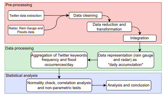
We extracted Twitter data for analyzing the frequency of meteorological-related posts before flooding/non-flooding events and its correlation with physical–meteorological data, specifically, rain gauge and weather radar measures. A region comprising the lower part of the Tamanduateí river basin and data collected between January and March 2009 were considered in this study. The literature has demonstrated that Twitter data can be a valuable and cost-effective data source for improving situational awareness in a way that is not possible by conventional data sources.
Data Sources
- Tweets: Twitter’s Academic API;
- Floods: Extracted from Emergency Management Center (CGE);
- Radar: Department of Airspace Control (DECEA);
- Rain gauges: Cemaden pluviometers;
Statistical methods:
Normality tests
The Shapiro–Wilk (SW), and Anderson–Darling are examples of single-sample tests useful in identifying whether an observed sample was drawn from a population with a normal distribution. Furthermore, the Shapiro–Wilk and Anderson–Darling tests are highlighted as the best tests to check data normality.
The Shapiro–Wilk test determines a statistic SW that acts as a threshold for the rejection region:
\[SW=\frac{(\sum^n_{i=i} \ a_i x^{(i)})^2}{\sum^n_{i=i}\ (x_i - \overline{x})^2}\]where $\overline{x}$ is mean value computed from the sample set; $x^{(i)}$ is the $i$-th smaller element into the sample set; and $a_i$ is the $i$-th component of the vector that comes from $\frac{m^T V^{-1}}{ \sqrt{ m^TV^{-1} V^{-1}m } }$, considering $m = [m_1,\ldots,m_n]^T$ as the expected values with equivalent order and drawn from a standard normal distribution, and $V$ is the covariance matrix computed from $[m_1,\ldots,m_n]$. In order to compute the $p$-value, one needs to verify the theoretical distribution of $SW$.
Similarly, the Anderson–Darling test will check the adherence between a sample set and an expected distribution, for example, the Gaussian distribution. The statistic regarding this test is presented in Equation:
\[AD = \left( -n - \sum^n_{i=1} \ \frac{2n-1}{n} \left( \ln{F(x_i)}+ \ln \left(1-F(x_{n+1-i}) \right) \right) \right) ^{\frac{1}{2}}\]where $F$ is the cumulative distribution function.
Correlation tests
Beyond the above-presented single-sample tests, the correlation and two independent samples tests help verify the relationship between variables and sets of observations. The Spearman’s rank correlation and Mann–Whitney are examples of tests applied to such cases.
Concerning the Spearman’s rank correlation, for a given set: ${ (x_i,y_i) : i=1,\ldots,n }$ with paired observations according to the variables $X$ and $Y$, the following~measure is computed: \(\rho = 1 - \frac{6 \sum (R(x_i)-R(y_i)) ^2}{n(n^2-1)}, \ d_i=R(X_i)-R(Y_i),\) where $R(\cdot)$ returns the rank of each observation according to the input variable. $\rho$ values closer to $-1$ or $1$ indicate intense direct or indirect correlation, respectively, between the compared variables~ In addition, the statistic $\displaystyle z = \rho \sqrt{\frac{n-2}{1-\rho^2}}$ follows a Student’s $t$-distribution with $n-2$ degrees of freedom. Consequently, we may use such a relation to compute the $p$-value, as the probability of values equal or larger than $z$, and then check the significance of $\rho$ in rejecting the null hypothesis of no correlation between the variables.
Results
All the codes and statistical results can be accessed here.
There were 166 traffic blocks due to floods in Tamanduateí basin in the period from January to March 2019, of which 89 were within a 2km radius from the selected rain gauges. Furthermore, initially, we had 17,493, 89,114 and 79,896 tweets in the neighborhood of 812A, 833A, and 857A rain gauges, respectively. After filtering the data based on a list of keywords, were found 139, 548, and 492 tweets on the abovementioned rain gauges, respectively. The number of selected tweets was about $0.65\%$ of the entire database. The graph depicting the data from the three analyzed points can be found in Figure:
The findings suggest that, in this case study, there is a weaker statistical relationship between extreme hydrological events and social media data when the volume of data is smaller. This is supported by the calculated p-values from the Spearman’s correlation for the 812A being smaller than those for the 833A and 857A gauges.
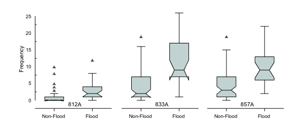
For further analysis of the relevance of geolocated tweets for flood detection, we counted the number of times that the keywords in filtered tweets appeared and performed a statistical comparison between the frequency of times that the keywords appeared on flood days and non-flood days. The result shows that the keyword frequency on flood days is superior to that on non-flood days:
The Mann–Whitney $U$ test was applied to verify the difference between flood days and non-flood days in the distribution of the (frequency of) keywords. The obtained $p$-values for 812A, 833A, and 857A were $1.267\times 10^{-5}$, $4.200\times 10^{-6}$, and $6.153 \times 10^{-7}$, respectively. These results make the differences already highlighted in boxplot figure.
Conclusion
This study makes a valuable contribution by rigorously demonstrating the statistical significance of tweets containing words related to hydrological extremes. By applying multiple tests of normality and non-parametric hypotheses, we have established a clear relationship between such tweets and extreme weather events. Our findings have important practical implications, particularly in the context of the significant economic and logistical losses caused by flooding. Furthermore, this research extends the existing literature on this topic and offers contributions for the development of technological tools to better address the challenges posed by flooding and its detrimental impacts.


